graph algorithms
Preface
I’m having a four-day break work, so I decided to finish the graphic algorithms convered in Introduction to Algorithm. They are the last part of this book. Throuthout my study, I plan to document this learning journey step by step, highlighting crucial concepts, and noting down all chanllenging and uncertain aspects for future review.
Basics
Representations of graphs
There are two types of graphs: directed and undirected, and for both of them, we can use a collection of adjacency lists or an adjacency matrix.
Let’s say V stands for vertices and E stands for edges so a graph G=(V,E). The number of V is |V| and so on E. If |E| is much less than |V|^2, a collection of adjacency lists is a better choice and otherwise, if |E| is close to |V|^2 an adjacency matrix is better.
Breadth-first search(BFS)
Given a vertex S in a graph G=(V,E), breadth-first search expolores all the rest of the vertices that are reachable to S systematically. This algorithm works on both directed and undirected graphs. Starting from source S, the algorithm first discovers all its neighbors and continues to use each neighbor as a new source to repeat this process until all vertices are found.
We use colors to keep track of the BFS: white means the vertex is never found, gray means it’s in process which is also called frontier, and black means it has been discovered.
Breath=first search constructs a breadth-first tree, whenever the search discovers a white vertex V in the course of scanning the adjacency list of a gray vertex U, the vertex V and the edge (U,V) are added to the tree. We say that U is the predecessor or parent of V in the breadth-first tree, and each reachable vertex from S has exactly one parent except the source S. If U is on the simple path in the tree from the root to vertex V, them U is an ancestor of V and V is a descendant of U.
BFS(G,S)
    for each vertex U belongs to G.V-S // all vertices but S
        U.color == WHITE
        U.d = -1 // means infinity
        U.P = NIL
    S.color = GRAY
    S.d = 0
    S.P = NIL
    Q = EMPTY;
    ENQUEUE(Q,S)
    whilc Q != EMPTY
        U = DEQUEUE(Q)
        for each vertex V in G.Adj[U]  //search the neighbors of U
            if V.color == WHITE        // is V being discovered first?
                V.color = GRAY
                V.d = U.d + 1;
                V.P = U
                ENQUEUE(Q,V)          // V is no on the frontier.
        U.color = BLACK               // U is behind the frontier.
- V.color is the color of V: WHITE, GRAY, or BLACK.
- V.d holds the distance from the source vertex S to V, as computed by the algorithm.
- V.P is V’s predecessor in the breath-first tree. If V has no predecessor then V.P = NIL.
Define the shortest-path distance 𝛅(S,V) from S to V as the minimum number of edges in any path from vertex S to vertex V.
-
Let G=(V,E) be a directed or undirected graph, and let S belongs to V be an arbitrary vertex. Then, for any edge (U,V) belongs to E: 𝛅(S,V) <= 𝛅(S,U) + 1.
-
Let G=(V,E) be a directed or undirected graph, and suppose that BFS is run on G from a given source vertex S belongs to V. Then, for each vertex V belongs to V, the value V.d computed by BFS satifies V.d >= 𝛅(S,V) at all times, including at termination.
-
Suppose that during the execution of BFS on a graph G=(V,E), the queue Q contains the verices <V1,V2,V3…Vr>, where V1 is the head of Q and Vr is the tail. Then, Vr.d <= V1.d + 1 and Vi.d <=V(i+1).d for i=1,2,…,r-1.
-
Suppose that vertices Vi and Vj are enqueued during the execution of BFS, and that Vi is enqueued before Vj. Then Vi.d<=Vj.d at the time that Vj is enqueued.
-
Let G=(V,E) be a directed or undirected graph, and suppose that BFS is run on G from a given vertex s belongs to V. Then, during its execution, BFS discovers every vertex v belongs to V that is reachable from the source s, and upon termination, v.d = 𝛅(S,V) for all v belongs to V. Moreover, for any vertex v!= s that is reachable from s, one of the shortes paths from s to v is a shortes path from s to v.P followed by the edge (v.P,V).
Predecessor subgraph
GP = (VP,EP) of G=(V,E), where
VP = {v belongs to V:VP!=NIL} and {S} EP = {(vP,v):v belongs to VP-{S}}
|EP| = |VP|-1
- When applied to a directed or undirected graph G=(V,E), prodcedure BFS constructs P so that the predecessor subgrapth GP=(VP,EP) is a breadth-first tree.
The PRINT-PATH procedure prints out the vertices on a shortest path from s to v provided that BFS has already construted a breadth-first tree.
PRINT-PATH(G,s,v)
    if v==s
        print s
    elseif v.P == NILL
        print "no path from so to v exists"
    else PRINT-PATH(G,s,v.P)
        print v
Depth-first search
DFS(G)
    for each vertex u belongs to G.V
        u.color = WHITE
        u.P = NIL
    time = 0 //gloabl time counter
    for each vertex u belongs G.V
        if u.color == WHITE
            DFS-VISIT(G,u)

DFS-VISIT(G,u)
    time = time + 1
    u.d = time
    u.color = GRAY
    for each vertex v in G.Adj[u]
        if v.color == WHITE
            v.P = u
            DFS-VISIT(G,v)
    time = time + 1
    u.f = time
    u.color = BLACK
- u.d is when the first time this vertex is found.
- u.f records when the search finishes examining u’s adjacency list.
- u.d and u.f are integers between 1 and 2|V|.
- u.d < u.f
- Vertex u is WHITE before time u.d, GRAY between time u.d and time u.f, and BLACK thereafter.
- DFS supports both undirected and directed graphs.
Properties of Depth-first Search
In any depth-first search of a (directed or undirected) graph G = (V,E), for any two vertices u and v, exactly one of the following tree conditions holds:
-
the intervals [u.d,u.f] and [v.d,v.f] are entirely disjoint, and neither u nor v is a descendant of the other in the depth-first forest.
-
the interval [u.d,u.f] is contained entirely within the interval[v.d,v.f], and u is a descendant of v in a depth-first tree, or
-
the interval [v.d,v.f] is contained entirely within the interval [u.d,u.f], and v is a descendant of u in a depth-first tree.
-
Vertex v is a proper decendant vertex u in the depth-first forest for a (directed or undirected) graph G if and only if u.d < v.d < v.f < u.f.
-
In a depth-first forest of a (directed or undirectd) graph G=(V,E), vertex v is a descendant of vertext u if and only if at the time u.d that the search discovers u, there is a path from u to v consisting entirely of white vertices.
Classification of edges
The depth-first forest GP produced by a depth-first on graph G an contain four types of edges:
-
Tree edges are edges in the depth-first forest GP. Edge(u,v) is a tree edge if v was first discovered by exploring edge(u,v).
-
Bach edges are those edges(u,v) connecting a vertex u to an ancestor v in a depth-first tree. We consider self-loops, which may occur in directed graphs, to be back edges.
-
Forward edges are those nontree edges(u,v) connecting a vertex u to a proper descendant v in a depth-first tree.
-
Cross edges are all other edges. They can go between vertices in the same depth-first tree, as long as one vertex is not an ancestor of the other, or they can go between vertices in different depth-first trees.
The key idea is that when an edge(u,v) is first explored, the color of vertex v says something about the edge:
- WHITE indicates a tree edge,
- GRAY indicates a back edge, and
- BLACK indicates a forward or cross edge. An edge(u,v) is a forward edge if u.d < v.d and a cross edge if u.d > v.d.
- In a depth-first search of an undirected graph G, every edge of G is either a tree edge or a back edge.
Topological sort
DAG: directed acyclic graph.
TOPOLOGICAL-SORT(G)
    call DFS(G) to compute finish times v.f for each vertex v as each vertex is finished, insert it onto the front of a linked list.
    return the linked list of vertices.
-
A directed graph G is acyclic if and only if a depth-first search of G yields no back edges.
-
TOPOLOGICAL-SORT produces a topological sort of the directed acyclic graph provided as its input.
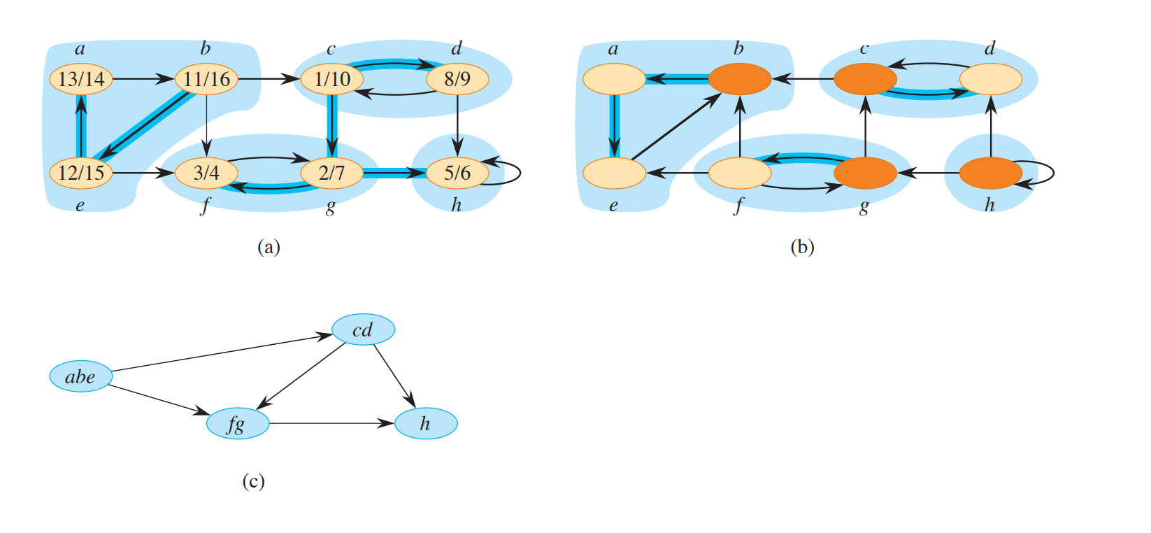
Strongly connected components
A strongly connected component of a directed graph G=(V,E) is a maximal set of vertices C belongs to V such that for every pair of vertices u,v belong to C, both u~>v and v~>u, that is, vertices u and v are reachable from each other.
The transpose of G is used to find the strongly connected components of G.
GT = (V,ET), where ET = {(u,v):(v,u) belongs to E}. ET consists of the edges of G with their directions reversed.
A key property of the component graph G-SCC = (V-SCC,E-SCC) : Suppose that G has strongly connected components C1,C2…Ck. The vertex set V-SCC is {v1,v2,…,vk}, and it contains one vertex vi for each strongly connected component Ci of G. there is an edge (vi,vj) belongs to E-SCC.
It’s not easy to understand this property, but there is a digram to explian this well. (c) is the component graph we are talking about here.
STRONGLY-CONNECTED-COMPONENTS(G)
    call DFS(G) to compute finish times u.f for each vertex u
    create GT
    call DFS(GT), but in the main loop of DFS, consider the vertices in order of decreasing u.f
    out put the vertices of each tree in the depth-first forest formed in last step as a separate strongly connected component.
- Let C and C’ be distinct strongly connected components in directed graph G = (V,E), let u,v beong to C, let u’,v’belong to C’, and suppose that G contains a path u~>u’. THe G cannot also contain a path v’~>v.
The notation for discovery and finish times extends to sets of vertices. For a subset U of vertices, d(U) and f(U) are the earliest discovery time and latest finish time, repectively, of any vertex in U:d(U)=main{u.d:u belongs to U} and f(U) = max{u.f:u belongs to U}.
-
Let C and C’ be distinct strongly connected components in directed graph G = (V,E). Suppose that there is an edge(u,v) belongs to E, where u belongs to C’ and v belongs to C. Then f(C’)>f(C).
-
Let C and C’ be distinct strongly connected components in directed graph G = (V,E), and suppose that f(C)>f(C’). Then ET contains no edge(v,u) such that u belongs to C’ and v belong to C.
-
The STRONGLY-CONNECTED-COMPONENTS procedure correctly computes the strongly connected components of the directed graph G provided as its input.
Minimum Spanning Trees
For an undirected graph G = (V,E), and for each edge(u,v) belongs E, a wight w(u,v) specifis the cost to connect u and v. The goal is to find an acyclic subset T belongs to E that connects all of the vertices and whos total wgight is minimized:
w(T) = w1(u1,v1)+w2(u2,v2)+…+(wr,vr), for each (ui,vi) belongs to T.
Growing a minimum spanning tree
GENERIC-MST(G,w)
    A = EMPTY
    while A does not form a spanning tree
        find an edge(u,v) that is safe for A
        A = A merge {(u,v)}
    return A
The generic method manages a set of A of edges, which grows the minimum spanning tree one edge at a time, maintaining the following loop invariant:
Prior to each iteration, A is a subset of some minimum spanning tree.
The tricky part is, of course, finding a safe edge.
definitions
- cut(S,V-S): A cut(S,S-V) of an undirected graph G=(V,E) is a partition of V.
- cross: We say that an edge(u,v) belongs to E crosses the cut(S,V-S) if one of its endpoints belongs to S and the other belongs to V-S.
- A cut respects a set A of edges if no edge in A crosses the cut.
- A edge is a light edge crossing a cut if its weight is the minimum of any edge corssing the cut. More generally, we say that an edge is a light edge satisfying a given property if its weight is the minimum of any edge satisfying the property.
A Theorem
- Let G=(V,E) be a connected, undirected graph with a real-valued weight function w defined on E. Let A be a subset of E that is included in some minimum spanning tree for G, let (S,S-V) be any cut of G that respects A, and let (u,v) be a light edge crossing (S,S-V). Then, edge (u,v) is safe for A.
A Corollary
Let G=(V,E) be a connected, undirected graph with a real-valued weight function w defined on E. Let A be a subset of E that is included in some minimum spanning tree for G, and let C=(Vc,Ec) be a connected component(tree) in the forest GA = (V,A). If (u,v) is a light edge connecting C to some other component in GA, then (u,v) is safe for A.
The algorithms of Kruskal and Prim
Kruskal’s algorithm
MST-KRUSKAL(G,w)
    A = EMPTY
    for each vertex v belong to G.V
        MAKE-SET(v)
    create a single list of the edges in G.E
    sort the list of edges into monotonically increasing order by weight w
    for each edge (u,v) taken from the sored list in order
        if FIND-SET(u) != FIND-SET(v)
            A = A merge {(u,v)}
            UNION(u,v)
    return A
Prim’s algorithm
MST-PRIM(G,w,r)
    for each vertex u belongs to G.V
        u.key = infinity
        u.P = NIL
    r.key = 0
    Q = EMPTY
    for each vertex u belongs to G.V
        INSERT(Q,u)
    while Q is not EMPTY
        u = EXTRACT-MIN(Q)
        for each vertex v in G.Adj[u]
            if v belongs to Q and w(u,v)<v.key
                v.P = u
                v.key = w(u,v)
                DECREASE-KEY(Q,v,w(u,v))
- r is the root of the minimum spanning tree.
- v.key is the minimum weight of any edge connecting v to a vertex in the tree.
- v.P manes the parent of v in the tree.
Single-Source Shortest Paths
Given a graph G=(V,E), find a shortest path from a given source vertex s belongs to V to every vertex v belongs to V.
- Given a weighted, directed graph G=(V,E) with weight function w: E->R, let p=<v0,v1…,vk> be a shortest path from vertex v0 to vertex vk and , for any i and j such that 0<=i<=j<=k, let pij = <vi,v(i+1),….,vj> be the subpath of p from vertex vi to vertext vj. Then pij is a shortest path from vi to vj.
A shortest path cannot contain a negative-weight cycle. Nor can it contain a positive-weight cycle, since removing the cycle from the path produces a path with the same source and destination vertices and a lower path weight. You can also remove a 0-weight cycle from any path to produce another path whose weihgt is the same. Therefore, that any sortest path contains at most |V|-1 edges.
A shortest-paths tree rooted at s is a directed subgraph G’=(V’,E’), where V’ belongs to V and E’ belong E, such that:
- V’ is the set of vertices reachable from s in G,
- G’ forms a rooted tree with root s, and
- for all v belongs to V’, the unique simple path from s to v in G’ is a shortest path from s to v in G.
Shortest paths are not necessarily unique, and neither are shortest path trees.
INITIALIZE-SINGLE-SOURCE(G,s)
    for each vertex v belongs to G.V
        v.d = infinity
        v.P = NIL
    s.d = 0
- v.d is an upper bound on the weight of a shortest path from source s to v. We call v.d a shortest-path estimate.
 RELEAX(u,v,w)
    if v.d > u.d + w(u,v)
        v.d = u.d + w(u,v)
        v.P = u
- Triangle inequality: For any edge(u,v) belongs to E, we have 𝛅(s,v) <= 𝛅(s,u) + w(u,v)
- Upper-bound property: We always have v.d>=𝛅(s,v) for all vertices v belongs to V, and once v.d achives the value 𝛅(s,v), it never changes.
- No-path property: If there is no path from s to v, then we always have v.d=𝛅(s,v)=infinity
- Convergence property: If s~u->v is a shortest path in G for some u,v belong to v, and if u.d = 𝛅(s,u) at any time prior to relaxing edge (u,v), then v.d=𝛅(s,v) at all times afterward.
- Path-relaxation property:If p=<v0,v1,…vk> is a shortest path from s=v0 to vk, and the deges of p relaxed in the order (v0,v1),(v1,v2)…(v(k-1),vk), then vk.d=𝛅(s,vk).
- Predeccssor-subgraph property: Once v.d=𝛅(s,v) for all v belongs to V, the predecessor subgraph is shortest-paths tree rooted at s.
The Bellman-Ford algorithm
 BELLMAN-FORD(G,w,s)
    INITIALIZE-SINGLE-SOURCE(G,s)
    for i = 1 to |G.V|-1
        for each edge(u,v) belongs to G.E
            RELAX(u,v,w)
    for each edge(u,v) belongs to G.E
        if v.d > u.d + w(u,v)
            return FALSE
    return TRUE
The algorithm returns TRUE if and only if the graph contains no negative-weight cycles that are reachable from the source.
Single-source shortest paths in directed acyclic graphs
DAG-SHORTEST-PATHS(G,w,s)
    topologically sort the vertices of G
    INITIALIZE-SINGLE-SOURCE(G,s)
    for each vertex u belongs to G.V, taken in topologically sorted order
        for each vertex in G.Adj[u]
            RELAX(u,v,w)
Dijkstra’s algorithm
Given a weighted directed graph G=(V,E): w(u,v)>=0 for each edge(u,v) belongs to E.
DIJKSTRA(G,w,s)
    INITIALIZE-SINGLE-SOURCE(G,s)
    S = EMPTY
    Q = EMPTY
    for each vertex u belongs to G.V
        INSEART(Q,u)
    while Q!=EMPTY
        u = EXTRACT-MIN(Q)
        S = S merge {u}
        for each vertex v in G.Adj[u]
            RELAX(u,v,w)
            if the call of RELAX decreased v.d
                DECREASE-KEY(Q,v,v.d)
Q is a min-prority queue Q of vertices, keyed by their d values.
The end
I think it’s enough for my work, and maybe later I’ll continue this.